3D-ΔPDF with Tb5Ru6Sn18 Data#

This tutorial demonstrates how to use the volume slicer’s Transform tab in NeuXtalViz to calculate a 3D-ΔPDF from normalized TOPAZ Tb5Ru6Sn18 volume data collected at room temperature (293 K), using a no-sample measurement as the background. The reciprocal-space steps show the (h,k,l=2) slice; the final real-space 3D-ΔPDF shows the (x,y,z=0) slice.

Step 1: Load the Room-Temperature Data#

Open NeuXtalViz and navigate to the Volume Slicer tab.
Load the normalized NeXus file for the 293 K dataset, naming it “293K”.
Set the slice axis value to L = 2.0.

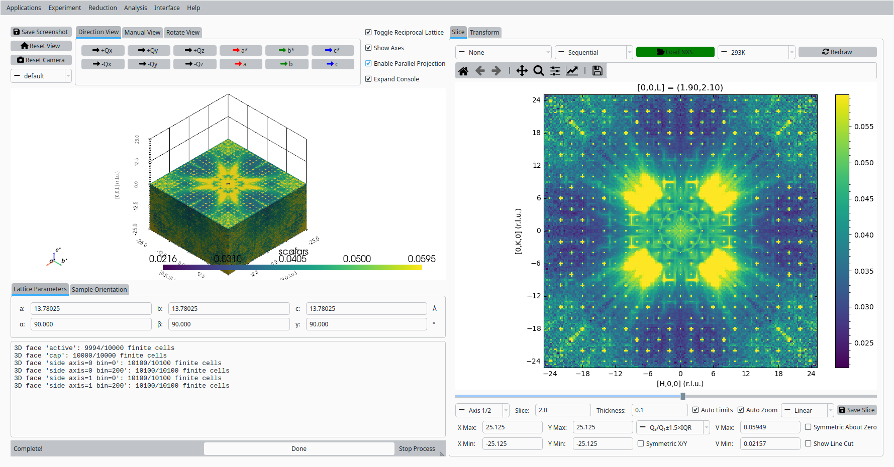
../_images/TbRuSn_deltaPDF_load_293K.png — Load the room-temperature Tb5Ru6Sn18 data at L = 2.#

Step 2: Load the No-Sample Background Data#

Load the normalized NeXus file for the no-sample background, naming it “bkg”.
Set the slice axis value to L = 2.0.

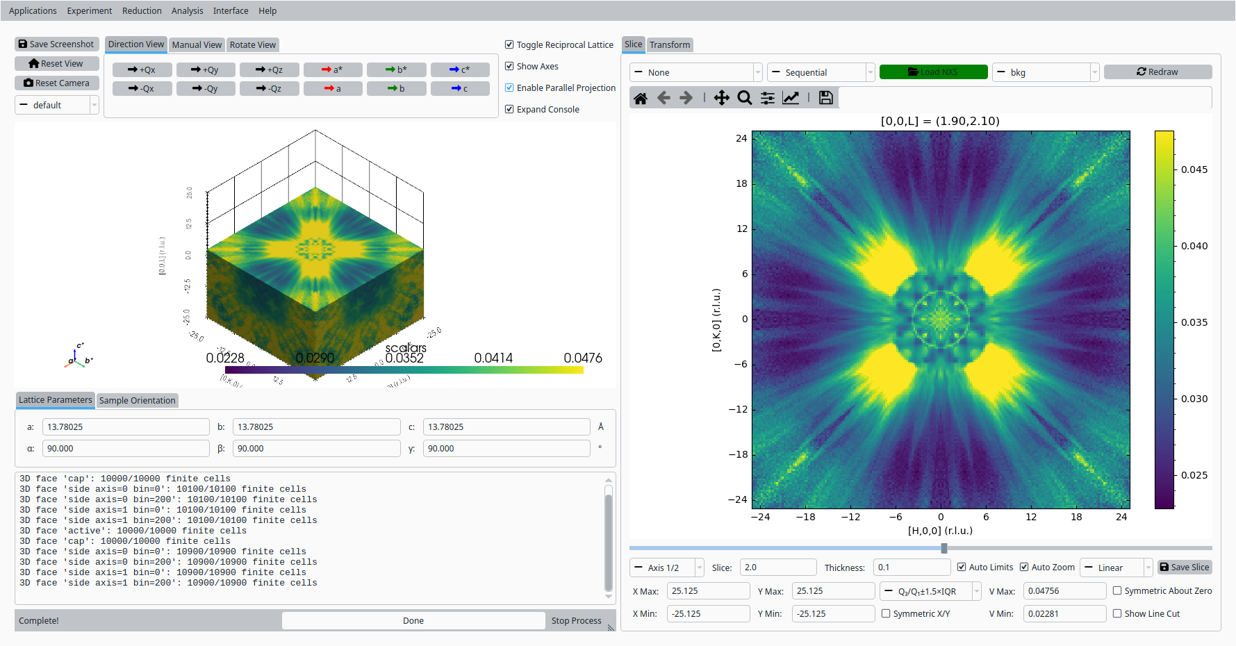
../_images/TbRuSn_deltaPDF_load_bkg.png — Load the no-sample background data at L = 2.#

Step 3: Subtract the No-Sample Background#

Switch to the Transform tab.
In the arithmetic panel, select “293K” as workspace A and “bkg” as workspace B.
Name the output “subtracted” and run the subtraction.

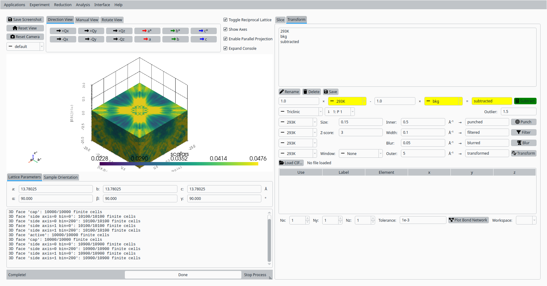
../_images/TbRuSn_deltaPDF_subtract.png — Subtract the no-sample background from the room-temperature data.#

Step 4: View the Subtracted Data#

Switch back to the Slice tab.
Select “subtracted” in the workspace combo.
Set the slice axis value to L = 2.0.
Set the color limits to V Min = 0 and V Max = 1e-2.

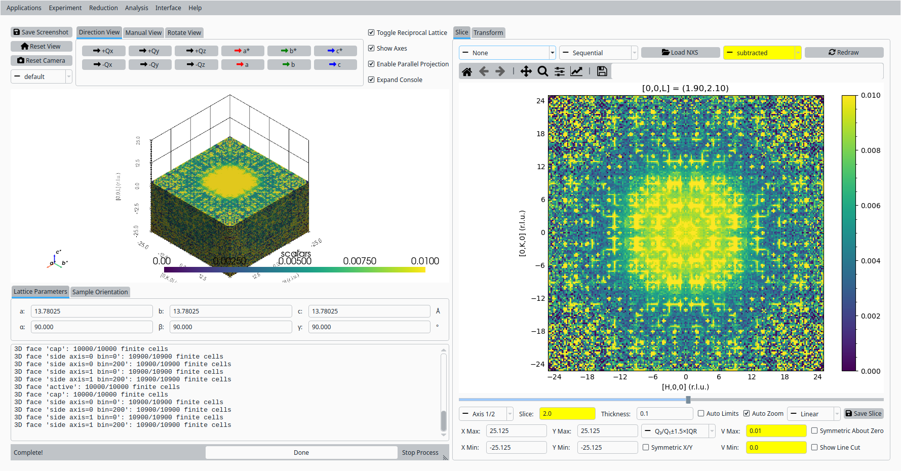
../_images/TbRuSn_deltaPDF_view_subtracted.png — View the subtracted reciprocal-space data at L = 2.#

Step 5: Punch the Bragg Peaks#

Switch back to the Transform tab.
Select the “Cubic” crystal system and space group 225 (Fm-3m).
Select “subtracted” as the input workspace, set the punch size to 0.25 (keeping the default inner radius), and run the punch.

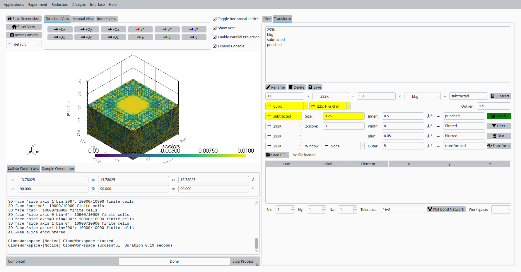
../_images/TbRuSn_deltaPDF_punch.png — Punch out the Bragg peaks and low-Q region.#

Step 6: View the Punched Data#

Switch back to the Slice tab.
Select “punched” in the workspace combo to see the punched-out regions at L = 2.

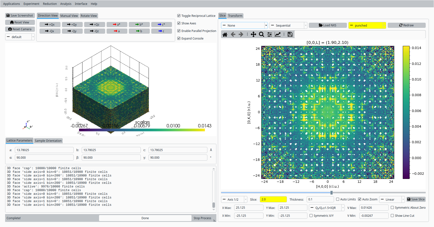
../_images/TbRuSn_deltaPDF_view_punched.png — View the punched reciprocal-space data at L = 2.#

Step 7: Fill the Punched Regions#

Switch back to the Transform tab.
Select “punched” as the input workspace, name the output “filled”, set the blur size to 0.1, and run the blur.

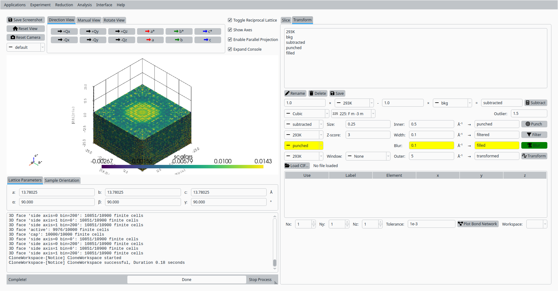
../_images/TbRuSn_deltaPDF_fill.png — Fill the punched regions with a NaN-Gaussian blur.#

Step 8: View the Filled Data#

Switch back to the Slice tab.
Select “filled” in the workspace combo to see the gaps closed in at L = 2.

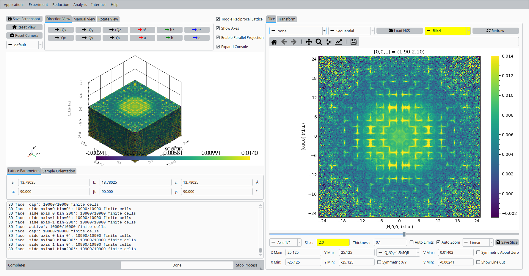
../_images/TbRuSn_deltaPDF_view_filled.png — View the filled reciprocal-space data at L = 2.#

Step 9: Calculate the 3D-ΔPDF#

Switch back to the Transform tab.
Select “filled” as the input workspace, choose the “Lorch” apodization window (keeping the default outer Q), and calculate the 3D-ΔPDF.

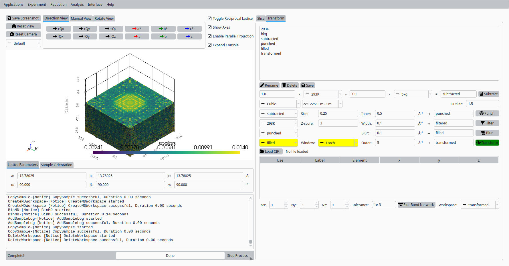
../_images/TbRuSn_deltaPDF_transform.png — Calculate the 3D-ΔPDF.#

Step 10: View the 3D-ΔPDF#

Switch back to the Slice tab.
Select “transformed” in the workspace combo.
Set the slice axis value to Z = 0.0 (the transformed result is real-space).
Set the color limits to V Min = -100 and V Max = 100.

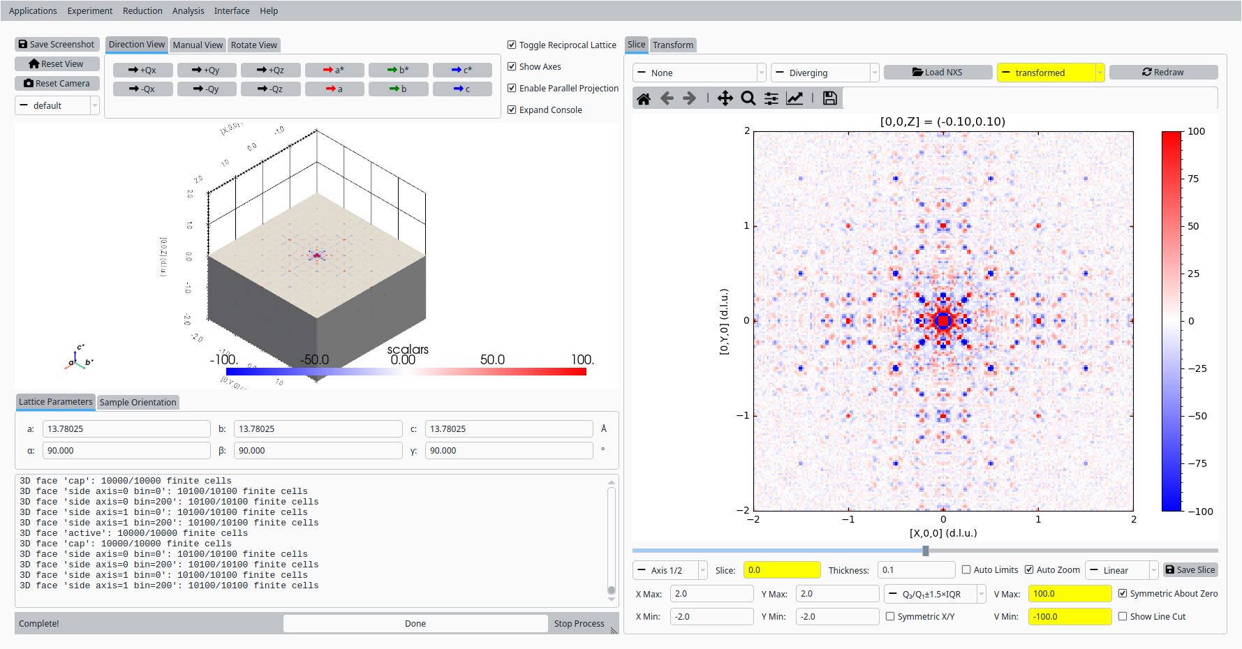
../_images/TbRuSn_deltaPDF_view_pdf.png — View the resulting 3D-ΔPDF at Z = 0.#